Auto-Encoding Variational Bayes
Variational Inference
I realized there is a lack of educational resources that concentrate on the theory of variational inference in this platform. If you’re interested in the math behind variational inference, or more generally speaking probabilistic programming, you may find this post useful.
According to Bayes rule,

where p(z|x) denotes posterior, p(x|z) denotes likelihood and p(x) denotes evidence, also called marginal likelihood. Computing the posterior is known as inference, but inference in some cases is analytically intractable because evidence, which is represented by the integration ∫p(x,z)dz, is a very high dimensional distribution, and it’s hard to draw samples from. Additionally, even if we’re able to estimate evidence accurately, we might need to compute other integrals. For instance,

KL Divergence
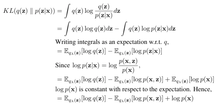
Variational inference handles the posterior computation as an optimization problem. Specifically, we choose a member of a family q(z), which is the variational distribution, and minimize the KL divergence from q(z) to the underlying true distribution, p(z|x). Once the optimization has been solved and q(z) is estimated, we handle inference using q(z) in place of p(z|x).

KL divergence measures how one distribution is different from another. If q(z) and p(z|x) are identical, then KL divergence is 0. Otherwise, it ranges between 0 and inf. It is always non-negative.
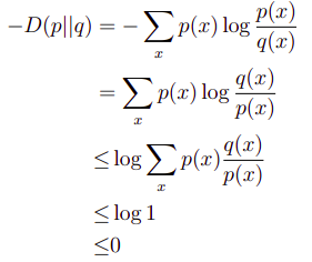
Proof KL divergence must always be non-negative. We show here the negative of KL divergence is always less than or equal to 0,

Evidence Lower Bound (ELBO)
KL divergence is dependent on an intractable objective: log p(x), which is the log probability of data. Since minimizing the KL divergence is equivalent to maximizing evidence lower bound (ELBO), we optimize ELBO instead, which is the negative of KL divergence plus the log probability of data,

First term in the Equation expresses energy and the second term (with the minus sign) is the entropy of q. The energy encourages q to place high mass on where the model puts high probability that is p(x,z), whereas the entropy acts as a regularizer, encouraging q to spread mass to avoid concentrating to one location.
ELBO sets a lower bound on the log probability of data: log p(x)≥L(λ). We can prove this using Jensen’s inequality which states that for any convex function f: f(E[x]) ≤ E[f(x)]. The opposite of this statement holds true for any concave function f. Since log is strictly concave,

ELBO can also be written as,

Instead of maximizing ELBO, we minimize the negative of ELBO to update the model parameters λ,

The first term in the objective function is the expected negative log-likelihood (NLL) and the second term is the regularizer: the KL divergence. NLL encourages the model to generate realistic output. If the model output isn’t realistic, it incurs a large cost in the loss function, whereas the KL divergence acts as a regularizer and measures the information loss when representing true posterior with a variational approximate.
Reparameterization Trick
Reparameterization trick is essential in order to backpropogate by taking the gradients of the objective function and updating the model parameters. We draw each latent variable z from a distribution q(z) learned by a model with parameters λ and we want to be able to take derivatives of ELBO with respect to λ, but backpropogation cannot flow through a random node.

Note: Terminology in the field is a bit sloppy, and you will see q(z) and q(z|x) are used interchangeably in the literature.
Reparameterization trick forces our samples to deterministically depend on the parameters of the approximate distribution i.e., instead of saying z is sampled from q(z|x) which is a univariate Gaussian under the simple assumption: z ∼ N (µ, σ^2 ), we are now describing z as a function that takes parameters (ε, (µ, σ)), where ε is an auxilary variable with independent marginal p(ε).
While doing backpropogation, all we need is to take the partial derivatives with respect to µ and σ, and ε allows us to sample while keeping the sampling operation differentiable. With ⊙, we signify an element-wise multiplication,

Closed-form Solution
The key ingredient of Auto-Encoding Variational Bayes is to evaluate a closed-form solution for the KL divergence under the assumption of a specific variational distribution, and utilize reparameterization trick to backpropagate. However this approach becomes a bottleneck when implementing variational inference in a wide variety of models for two reasons: i) there is no closed-form solution of the gradient for the arbitrary variational family, ii)deriving a closed form solution on a model-by-model basis is a tedious process.
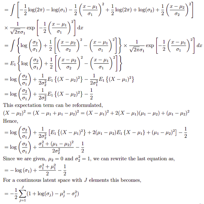
If we assume the variational distribution, q, is a univariate Gaussian with mean µ_1 and standard deviation σ_1, and the true posterior, p, is a univariate Gaussian with mean µ_2 and standard deviation σ_2, the KL divergence from q to p is,

After taking the log of Gaussian distributions, this can be rewritten as,

Substituting this in the objective function we have already defined above will provide,
